How to Strikethrough in Excel?

Strikethrough is a helpful formatting tool in Excel that lets you put a line through text or numbers to show they are no longer needed or are marked for deletion. It’s useful in task lists, editing documents, or managing data updates. Though it’s not as commonly used as bold or italic, it can be just as important when you want to visually mark something without deleting it completely.

What is Strikethrough?

Strikethrough is a formatting style that places a horizontal line through text or numbers, signaling that the content is no longer active or needed. It doesn’t delete the data; it simply highlights it as completed or outdated much like ticking off an item from a checklist. The item is still there, but you can see it’s been handled or is no longer needed.

Why Use Strikethrough in Excel?

There are many reasons to use strikethrough in Excel, especially if you’re working with checklists, tracking edits, or handling large data sets. Here are a few everyday examples:

1. To cross off completed tasks in a project tracker
2. To show which items have been canceled or replaced
3. To keep records of old data without deleting them
4. To mark changes during data reviews
5. To help visually filter or manage information

It’s a great way to make your spreadsheet look organized while keeping the original data intact.

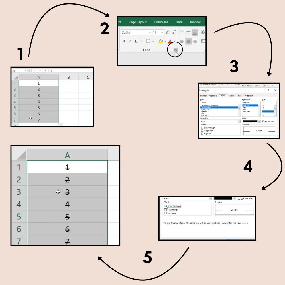
Method 1: Using the Format Cells Dialog Box

The most common way to apply strikethrough in Excel is by using the Format Cells window.

 

Here’s how:

1. Highlight the cell or group of cells where you want to apply the strikethrough effect.
2. Right-click on the selection
3. Click on Format Cells from the menu
4. In the Format Cells window, go to the Font tab
5. Check the Strikethrough option
6. Click OK

The selected text or numbers will now appear with a line through them. This method works for both individual cells and multiple selected cells.

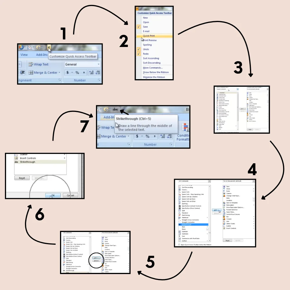
Method 2: Using the Excel Ribbon (Toolbar)

If you prefer using the toolbar (also called the Ribbon), you can add the strikethrough button there for quick access.

Here’s how you can do it:

1. Click the small downward arrow in the Quick Access Toolbar (top-left corner of Excel)
2. Choose More Commands
3. From the “Choose commands from” dropdown menu, select Commands Not in the Ribbon.
4. Scroll through the list and locate Strikethrough.
5. Click Add, then press OK to confirm.

Once added, the Strikethrough button will appear in your Quick Access Toolbar, making it quicker to apply. To use it, simply highlight the desired cell or range and click the icon—Excel will instantly apply the strikethrough formatting.

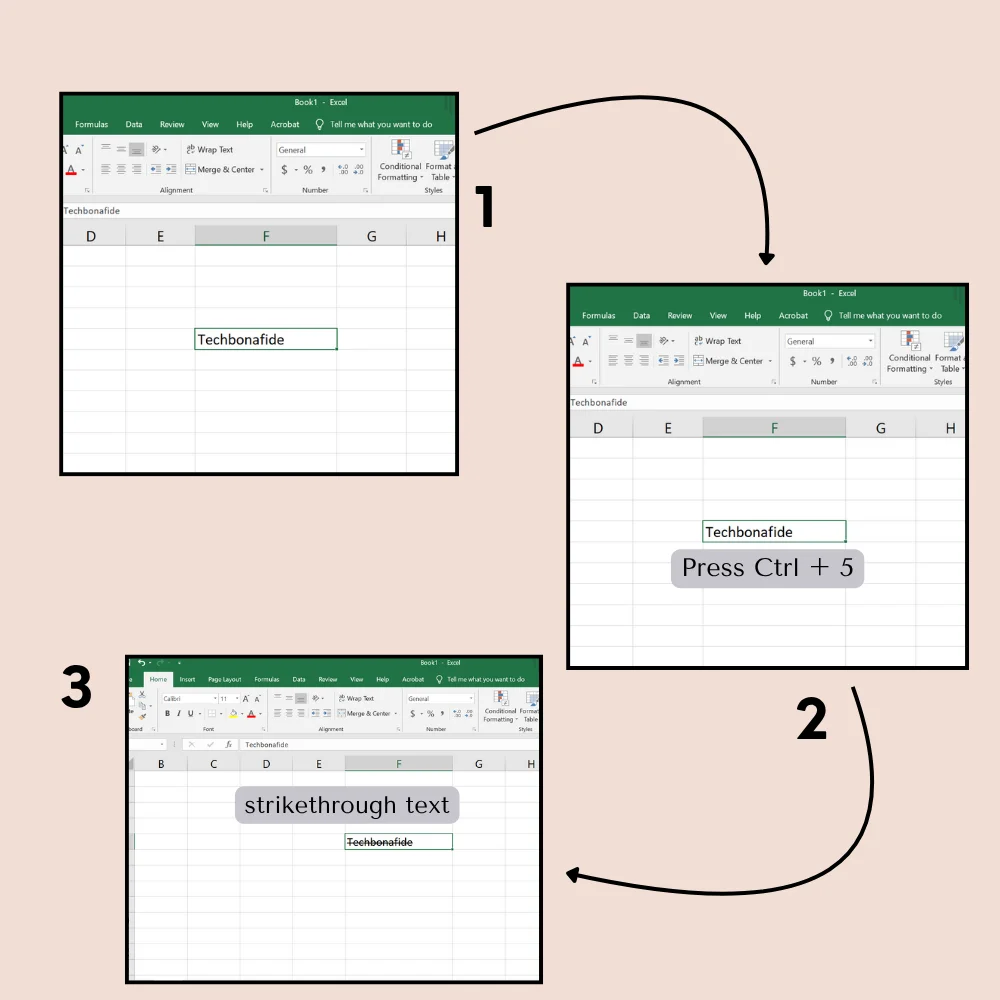
Method 3: Keyboard Shortcut for Strikethrough

One of the fastest ways to strikethrough text in Excel is by using a simple keyboard shortcut.

Shortcut: Ctrl + 5

How to use it?

• Click on the cell you want to apply the strikethrough to
• Press Ctrl and 5 at the same time
• The text in the cell will instantly get a line through it

This works in Excel on both Windows and Mac, though on Mac you may need to use Command (⌘) + Shift + X depending on your version.

This shortcut is especially useful when you’re working on large sheets and want to make quick edits without going through menus.

Method 4: Applying Strikethrough Through Conditional Formatting

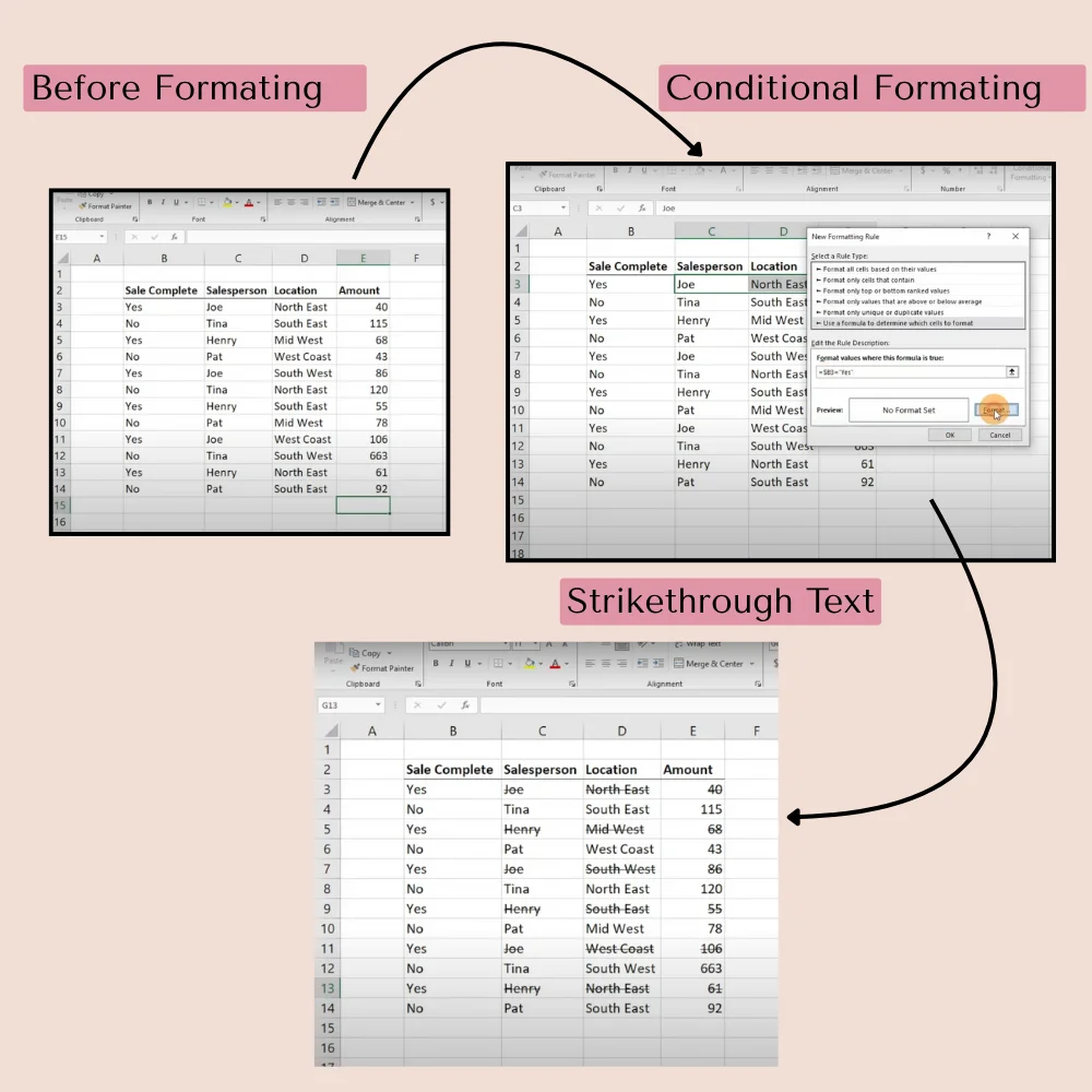
Conditional formatting allows you to apply formatting like strikethrough based on a rule. This is great if you want Excel to automatically cross out cells when a certain condition is met.

Here’s how to set it up?

1. Select the range of cells you want to apply the rule to
2. Go to the Home tab
3. Click on Conditional Formatting > New Rule
4. Select Use a formula to decide which cells to format from the list of rule types.
5. Enter a formula like this: =A1=”Done” (replace with your actual condition)
6. Click Format
7. In the Font tab, check Strikethrough, then click OK
8. Click OK again to apply

Now, whenever the cell contains “Done”, it will automatically be crossed out. You can customize the condition to suit your needs.

Method 5: Strikethrough Only Part of the Text in a Cell

Sometimes you may want to strikethrough just a portion of the text in a cell instead of the whole thing. Excel allows you to do that manually.

Here’s what to do?

1. Double-click the cell to edit it
2. Select the part of the text you want to strikethrough
3. Right-click and choose Format Cells
4. In the Font tab, check Strikethrough
5. Click OK

Only the selected part of the text will have a line through it. This is helpful when you want to show partial changes or edits within one sentence.

Method 6: Strikethrough in Excel Online

If you’re working with Excel in a web browser (Excel Online), some formatting features may be limited compared to the desktop version. The right-click Format Cells option doesn’t have strikethrough in the font settings.

But don’t worry you can still use a shortcut:

• Select the cell(s)
• Press Ctrl + 5 on your keyboard

This shortcut works in most browsers and will apply the strikethrough just like in the desktop version.

Bonus Tips for Using Strikethrough in Excel

Here are some extra pointers to make working with strikethrough smoother:

• Combine with other formats: You can use strikethrough along with bold, italic, or color to make your data more readable.
• Use filters: If you’re crossing off items in a list, apply a filter so you can hide or show only the items that are still active.
• Track revisions: In collaborative spreadsheets, strikethrough helps show what’s been changed without deleting anything, especially useful for financial or inventory records.
• Print-ready: Strikethrough formatting is printable, so you don’t lose your changes when you generate hard copies.

Final Thoughts

Strikethrough in Excel is a handy feature that helps you organize and manage data without removing it. Whether you’re updating task lists, marking completed items, or highlighting changes, it offers a clear visual cue while keeping original content intact. Once you start using it, you’ll find it makes tracking progress and edits much easier in your day-to-day Excel work.